 网站地图
网站地图

 下载:
下载:


-
当前数字化的测量手段蓬勃发展,测量精度逐步提升,应用也愈发广泛。其中激光测量系统,例如激光跟踪仪、激光雷达等在诸多领域得到了广泛应用[1-3]。特别是在航空、航天、船舶等大型的制造业领域,产品的尺寸越来越大,加工、装配等工艺的精度要求也越来越高[3-5], 其中激光测量系统得到了非常广泛的应用。在精密测量与大尺寸测量的问题中,测量系统获得的坐标通常不能直接应用于相关指标的计算与装配的分析,而是需要开展相应的测量误差分析与装配坐标系转换。激光测量系统的误差,通常设备会给出具体值,例如某型号激光跟踪仪的标称不确定度为15μm+6μm/m,即基础误差为15μm, 测量距离每增加1m, 其误差增加6μm。随着实际应用场景提出了越来越高的需求,仅仅是测距方向上的最大误差已经很难满足很多测量场景的测量设计与实施指导。测量不确定度在各个方向上的各向异性,即具体在测量空间的3维分布,对测量以及加工与装配实施中的重要精密指标确定已经产生了影响,甚至进一步对测量设备的布局提出了要求[6-11]。当前一系列的研究主要通过复杂的优化模型,例如迭代最近点法(iterative closest point, ICP)、奇异值分解法(single value decomposition, SVD)、蒙特卡洛(Monte Carlo, MC)数值估计等,来对变换参量进行优化,随后分析这一系列的模型中的误差传递,通过数值仿真的思路进行特定点的不确定度分析[6, 9-10, 12-16]。然而为了结合设备的状态与实测的场景,往往需要针对复杂的模型开展重复的大量优化计算,这无疑对现场测量带来了很大的不便。而计算获得的大量仿真点或者不确定度模型往往也需要与实际的特定点大量测量数据进行数据筛选、模型坐标变换匹配与误差比对。当前对于大量数据筛选依然主要为面向拟合目标的分析而非脱离应用的误差分析[17]。因此,需要提出以更高效的算法准确地筛选获取基于大量实测或者仿真点数据的最小包络模型,即不确定度模型。
孤立森林算法(isolated forest algorithm,IFA)是一种基于数据空间随机切分迭代的异常值检测方法。该算法通过随机超平面在数据空间内进行切分,并将切分后的子空间以二叉树进行数据结构构建。对每个子空间进行相同的随机切分并构成子树(分枝),直至每个分枝有且只有一个数据。通过在样本空间多次随机采样并构建系列数据树,形成数据森林。通过判定数据空间中每个点距离数据树根部的深度评估其异常程度,并据此进行数据筛选。该算法已经广泛应用于各领域的异常检测、数据清洗等过程[18-21]。粒子群优化(particle swarm optimization,PSO)算法是一种更偏重于群体智能的优化算法。其将待确定问题的集合作为一个粒子,并以粒子群模仿鸟群觅食的行为特征在解空间进行探索。每个粒子结合自我认知与群体经验交流,遵循相同的规则进行运动。区别于传统优化算法,该算法具备较强的跳出局部最优解的能力,并已经广泛应用于了函数优化、神经网络训练、决策、建模等诸多领域[13, 22-27]。
本文中的研究以激光跟踪仪系统为研究对象,以单点测量实验出发,引入了孤立森林算法对不确定度测量数据进行处理与分析,并采用粒子群优化算法进行最小包络椭球计算,高效快速准确地获取该设备的单点测量不确定度分布情况。该方法仅基于单点的测量数据,因此可以应用于各型号的激光跟踪仪以及激光雷达等其它激光球坐标测量系统的不确定度分布测试实验,甚至MC模型的仿真数据分析。以此为基础,可以通过测量与仿真数据分析获得3维空间内不同位置的不确定度分布,因此, 本研究具有进一步指导测量场景布局设计等重要意义。
-
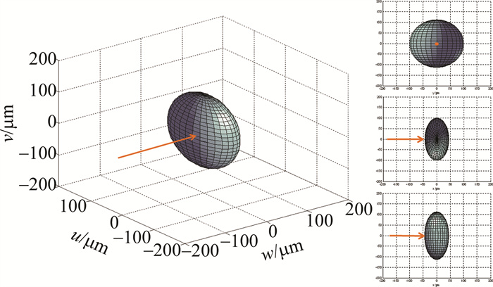
本文中的研究对象为Leica At-930激光跟踪仪。以测量位置靶球中心为原点可以建立不确定度椭球坐标系(uncertainty ellipsoid coordinate system,UCS),在此坐标系(w, u, v)下不确定度椭球包含的范围可以描述为方程:
$ E(w, u, v)=\frac{w^{2}}{a^{2}}+\frac{u^{2}}{b^{2}}+\frac{v^{2}}{c^{2}}-1 \leqslant 0 $
(1) 式中,w, u, v是测量点在UCS三坐标轴w, u, v上的坐标值,a,b,c分别是该不确定椭球的三轴半轴长。图 1为UCS下不确定度椭球示意图。
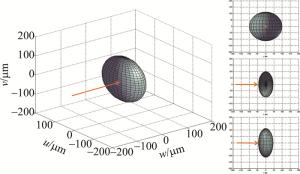
图 1 Schematic diagram of uncertainty ellipsoid under UCS
在实际测量中,靶球的位置会随着测量目标的变化而变化,即各测量点分别存在其独立的UCS,因此, 测量数据往往采用统一的基于跟踪仪的测量系统坐标系(measurement coordinate system,MCS)。对于任意UCS其坐标轴单位向量在MCS上可以描述为:
$ \left\{\begin{array}{l} \boldsymbol{u}=\left[\begin{array}{lll} \sin \alpha & -\cos \alpha & 0 \end{array}\right]^{\mathrm{T}} \\ \boldsymbol{v}=\left[\begin{array}{lll} \cos \beta \cos \alpha & \cos \beta \sin \alpha & -\sin \beta \end{array}\right]^{\mathrm{T}} \\ \boldsymbol{w}=\left[\begin{array}{lll} \sin \beta \cos \alpha & \sin \beta \sin \alpha & \cos \beta \end{array}\right]^{\mathrm{T}} \end{array}\right. $
(2) 式中,α为方位角,β为天顶角,w为测量的激光方向,v为w与z平面上垂直于w的方向,u为遵循右手定则垂直于w与v的方向。由UCS到MCS的旋转矩阵则可以描述为:
$ {}_{\operatorname{UCS}}^{\operatorname{MCS}} \boldsymbol{R}=[\boldsymbol{w}, \boldsymbol{u}, \boldsymbol{v}] $
(3) 图 2为激光跟踪仪MCS与坐标系UCS的转换示意图。
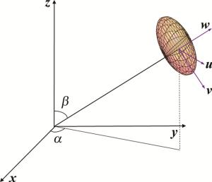
图 2 Coordinate system conversion of laser tracker between MCS and UCS
对于测量点P,在其位置构建的UCS在MCS上的位置矢量可以描述为:
$ ^{\operatorname{MCS}}_{\operatorname{UCS}} \boldsymbol{P}_{O}=\left[x_{0}, y_{0}, z_{0}\right] $
(4) 式中,x0,y0,z0为在该位置累积测量采样分布的期望,以其近似为理论靶球中心。据此两坐标系变换的变换矩阵可以描述为:
$ ^{\text {MCS}}_{\text {UCS}} \boldsymbol{T}=\left[ {\begin{array}{*{20}{c}} {_{{\rm{UCS}}}^{{\rm{MCS}}}\mathit{\boldsymbol{R}}}&{_{{\rm{UCS}}}^{{\rm{MCS}}}{\mathit{\boldsymbol{P}}_O}}\\ {\begin{array}{*{20}{c}} 0&0&0 \end{array}}&1 \end{array}} \right] $
(5) $ { }_{\text {MCS}}^{\text {UCS}} \boldsymbol{T}=\left[ {\begin{array}{*{20}{c}} {_{{\rm{UCS}}}^{{\rm{MCS}}}{\mathit{\boldsymbol{R}}^{\rm{T}}}}&{ - _{{\rm{UCS}}}^{{\rm{MCS}}}{\mathit{\boldsymbol{R}}^{\rm{T}}}{\kern 1pt} {\kern 1pt} _{{\rm{UCS}}}^{{\rm{MCS}}}{\mathit{\boldsymbol{P}}_O}}\\ {\begin{array}{*{20}{c}} 0&0&0 \end{array}}&1 \end{array}} \right] $
(6) 据此依据通用坐标系转换公式:
$ \left[\begin{array}{c} { }^{A} \boldsymbol{P} \\ 1 \end{array}\right]={ }_{B}^{A} \boldsymbol{T} \cdot\left[\begin{array}{c} { }^{B} \boldsymbol{P} \\ 1 \end{array}\right] $
(7) 式中,A, B作为通用坐标系表达均可以替换为MCS或UCS,据此任意测量位置在MCS下的累积采样位置数据均可以通过坐标变换转换为UCS下进行标准不确定度椭球的分布分析;而分析获得的不确定度椭球同样可以转换为MCS下测量场不同位置的椭球分布。
-
基于固定设备与采样点位的单点重复位置测量与基于蒙特卡洛等算法的单点位随机仿真测点均是获取单点位置不确定度分布的重要方法。这些方法可以获得对于单点的大量测量/仿真位置数据,实测过程中由于场地与设备等因素的扰动会获得极少数较大的误差点,而在算法仿真中同样会由于必要的扰动函数产生少量较大误差点。在进行不确定度包络椭球计算时,这些较大误差点会对包络计算形成干扰,使得最终获得的包络椭球过大。本研究中,引入了孤立森林算法来对测量/仿真数据进行采样筛选。
基于本课题问题研究,孤立森林算法模型可以通用化描述为{D, F, H, fs, rs, Nt, Nsub, nDFR},其中D={P1, P2, …, PN}为数据空间,包含所有的待分析筛选的数据,其数据个数为N,对于每个数据点P,其维度为d,在本研究问题中,D即为所有测量/仿真位置数据的集合,维度d=3;F={T1, T2, …, TNt}为孤立森林算法划分出的森林,其中T为森林中的独立数据树,Nt为每座森林中树的个数;对于每个数据树T包含集合Dsub={Pr, 1, Pr, 2, …, Pr, i…Pr, Nsub}的全部数据,并通过孤立函数fs划分为二叉树结构,Nsub为每棵树的数据个数,Pr, i为数据空间中随机出的第i个数据;Dsub为每棵树的数据集合,其为D的随机样本量是Nsub的子集;孤立函数fs可以描述为:
$ \left\{\begin{aligned} \boldsymbol{D}_{\mathrm{sub}, \mathrm{l}, h+1}=& f_{\mathrm{s}, \mathrm{l}}\left(\boldsymbol{D}_{\mathrm{sub}, h}, S_{\mathrm{r}, h}\right)=\left\{\boldsymbol{P}_{\mathrm{r}, i} \mid \boldsymbol{P}_{\mathrm{r}, i}\left(r_{d}\right) \leqslant\right.\\ &\left.S_{\mathrm{r}, h}, \boldsymbol{P}_{\mathrm{r}, i}\left(r_{d}\right) \in \boldsymbol{D}_{\mathrm{sub}, h}\right\} \\ \boldsymbol{D}_{\mathrm{sub}, \mathrm{r}, h+1}=& ∁\ \ \ _{{D_{\mathrm{sub}, h}}} \boldsymbol{D}_{\mathrm{sub}, \mathrm{l}, h+1} \end{aligned}\right. $
(8) 式中,Dsub, l, h与Dsub, r, h分别代表该数据树在距离根部深度为h(即h层)的左右数据子集;Sr, h为该数据树在h层数据孤立分割的标准,其取值为[min(Dsub, h), max(Dsub, h)]范围内的随机值;因为D为d维的数据集,在孤立分割时,取随机整数rd∈[1, d]作为分割判定时的比较维度,Pr, i(rd)即为数据Pr, i在比较维度rd下的数据分量。在筛选计算中, 将后续的Dsub, l, h+1, 或者Dsub, l, h+1分别作为新的子数据集Dsub, h+1, 采用孤立函数fs进行递归迭代划分,直到最终层次的Dsub样本量为1,即完成数据树的构建。H为每个数据点在森林中每个树上距离根部的深度的平均值的集合;rs为算法的筛选次数,即森林的个数;nDFR则为每次筛选时判定标准,即数据距离根节点的深度(deep from root, DFR),即当H(Pi) < nDFR时,Pi为较大误差点, 当被舍弃。最终经过孤立森林算法筛选后的数据空间D0则为后续不确定度椭球模型的数据基础。
-
通过坐标转换与数据筛选后的测量/仿真位置数据可以通过PSO基于(1)式进行最小包络椭球模型的建立。在UCS下,椭球中心为原点,因此最小包络的控制因素则为椭球三轴的半轴长。定义粒子X={a, b, c},解的搜索空间为3维。在解空间随机生成n个粒子,每个粒子Xi均为该系列数据的潜在一个包络椭球解。随着迭代时刻t的推进,每个粒子均在解空间以一定速度Vi运动探索以获取最优的包络解。每个粒子的运动规则遵循:
$ \begin{gathered} \boldsymbol{V}_{i, t+1}=\omega \cdot \boldsymbol{V}_{i, t}+c_{1} r_{1}\left(L_{i, t}-\boldsymbol{X}_{i, t}\right)+ \\ c_{2} r_{2}\left(\boldsymbol{G}_{t}-\boldsymbol{X}_{i, t}\right) \end{gathered} $
(9) $ \boldsymbol{X}_{i, t+1}=\boldsymbol{X}_{i, t}+\boldsymbol{V}_{i, t+1} $
(10) 式中,Xi, t与Vi, t为第i个粒子在t时刻的位置与运动速度;Li, t为第i个粒子到t时刻其个体运动轨迹中的最优解,代表着粒子的个体认知;Gt为t时刻所有粒子运动轨迹中的最优解,代表着粒子的群体交流与共识;ω为惯性因子,c1和c2为学习因子,控制着粒子向自身经验和群体经验学习的倾向,r1和r2为随机因子,为[0, 1]之间的随机数。在每次运动迭代完成后,粒子Xi, t均以适应值函数fe来进行评价,通常适应值越小,该粒子距离理论最优解越近。本研究中以包络椭球解的体积作为评价标准,因此对于粒子Xi={ai, bi, ci}:
$ f_{\mathrm{e}}\left(\boldsymbol{X}_{i}, r_{\mathrm{e}}\right)=\left\{\begin{array}{l} \frac{4}{3} {\rm{ \mathit{ π} }} a_{i} b_{i} c_{i},\left(n_{\mathrm{in}} \geqslant N_{0} \cdot r_{\mathrm{e}}\right) \\ -1,(\text {others}) \end{array}\right. $
(11) 式中,re为椭球模型对数据D0的包络比例,N0为D0中数据的个数,nin为D0中处于包络范围内的数据个数,可以描述为:
$ n_{\mathrm{in}}=\overset{N_0}{\underset{i}{\operatorname{argnum}}}\left(\boldsymbol{P}_{i}, E_{\boldsymbol{X}_{i}}\left(\boldsymbol{P}_{i}\right) \leqslant 0\right),\left(\boldsymbol{P}_{i} \in \boldsymbol{D}_{0}\right) $
(12) 式中,argnum函数的输出结果为满足后续条件的数据Pi个数,EXi(Pi)为点Pi代入粒子Xi条件下的包络椭球模型E(见(1)式)计算其相对于椭球包络面的位置。通过适应值函数,在每次粒子群运动迭代后对个体历史最优解Pi与全局最优解G进行更新:
$ \boldsymbol{L}_{i, t+1}=\left\{\begin{array}{l} \boldsymbol{X}_{i, t+1},\left(f_{\mathrm{e}}\left(\boldsymbol{L}_{i, t}\right)>f_{\mathrm{e}}\left(\boldsymbol{X}_{i, t+1}\right),\right. \\ \ \ \ \ \ \ \ \ \ \ \ \ \left.f_{\mathrm{e}}\left(\boldsymbol{X}_{i, t+1}\right) \neq-1\right) \\ \boldsymbol{L}_{i, t},(\text {others}) \end{array}\right. $
(13) $ \boldsymbol{G}_{t}=\overset{n}{\underset{i=1}{\operatorname{argmin}}}\left(\boldsymbol{L}_{i, t}, f_{\mathrm{e}}\left(\boldsymbol{L}_{i, t}\right)\right) $
(14) 式中,argmin函数的输出结果为使得适应值函数fe最小的粒子Li。
在本研究问题算法执行流程为对所有粒子在粒子空间进行随机位置初始化,通过(9)式~(14)式对每个粒子的运动位置与速度的迭代计算完成最优包络的探索。区别于传统优化问题,最小包络的探索在(11)式~ (13)式中存在对包络数据比例的判定,因此为实现优化探索的准确性与效率,需要选择合适的初始化粒子位置范围与粒子陷入过小包络模型局部位置后的扰动逃逸模型。粒子初始化位置为:
$ \boldsymbol{X}_{i}=\left(w_{\max }, u_{\max }, v_{\max }\right) \cdot r_{x}\left(l_{0}\right) $
(15) 式中,wmax,umax,vmax为UCS下所有点在三坐标轴下的绝对值极值,rx为[1, l0]范围的随机值,l0为空间放大系数。扰动逃逸函数在当前粒子无法满足包络要求时可以替代其位置更新函数,描述为:
$ \boldsymbol{X}_{i, t+1}=\boldsymbol{X}_{i, t} \cdot e_{\mathrm{s}}+\boldsymbol{V}_{i, t+1} \mid f_{\mathrm{e}}\left(\boldsymbol{X}_{i, t}\right)=-1 $
(16) 式中,es为逃逸系数。
-
研究采用LeicaAt-930激光跟踪仪以及3.81cm的跟踪仪靶球,进行固定机位与靶球位的单点多重数据测量采集,并将数据应用于孤立森林模型数据筛选与最小包络椭球求取,以验证模型的有效性。
-
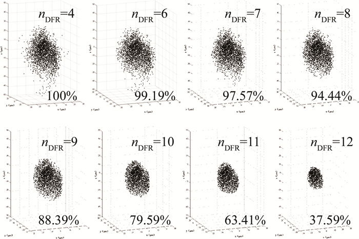
固定跟踪仪设备,在距离设备约4.7m的固定靶球位置的单点采集N=3091个位置坐标值。孤立森林筛选次数rs=10,森林中数据树的数目Nt=100,每棵树的数据量Nsub=256。由图 3可知,采样点云分布即为椭球型,但也能发现存在系列远离点云的少量误差较大点。nDFR=4时,保留采样点依然为100%,舍弃误差点数量为0,即所有点在数据树上的平均高度均大于4;当nDFR取为6和7时,依然存在少量误差较大点保留;当nDFR>8时,较大误差点已基本被去除,随着nDFR值增大,椭球周边点分布密度较小的区域也逐渐被去除,保留的采样点比例逐步减小。
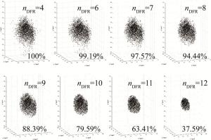
图 3 Screening results of the isolated forest under different DFR
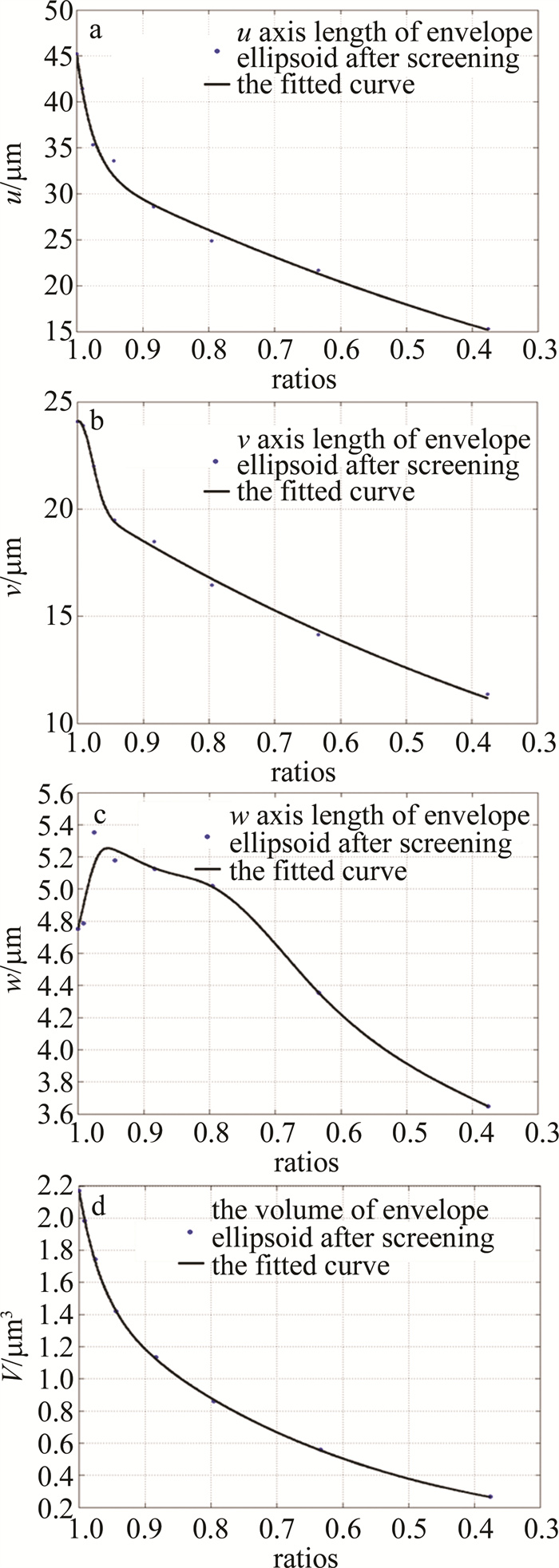
将筛选后的数据点进行三轴及椭球体积的包络椭球分析, re=0.99时的结果如图 4、图 5所示。图 4中百分比为筛选后有效数据占原全部数据的比例,轴长变化曲线均采用了双高斯拟合。筛选后有效数据比例由100%减小到约95%的过程,包络椭球u,v轴半轴长度减小速率较快,这说明较大误差点是分布在u,v轴方向离中心较远的位置。筛选保留比例减小到95%以下后,包络椭球u,v轴半轴长减小曲线符合高斯曲线,即去除掉较大误差点后,采样点在u,v两轴的密度分布为由中心向外的高斯分布。对于w轴,随着筛选后有效数据比例由100%减小到约95%,w轴半轴长随之增大,这是因为加大误差点是在在u,v轴方向离中心较远的位置,其在w轴上投影较小,过大的u,v轴长使得包络椭球更呈现扁而长宽的形状。随着误差较大点的去除,u,v轴长急剧减小,为使得中央高密度点云分布能够完成包络,w轴长会呈现增长的趋势。而随着有效比例到达95%到约80%,由于较大误差点已经基本被去除,w轴半轴长开始逐渐减小,但此时其减小的趋势远小于另外两轴,这是因为点云主要在u,v轴方向延伸分布,存在点云密度相对较低的包围区域,这些点的去除对w轴轴长的影响相对较小。随着比例减少到80%以下,点云的筛选到达核心区域,此时w轴轴长的减小同样符合高斯曲线,即在核心点云分布区域w轴方向点密度分布也是呈高斯分布。结合以上分析,孤立森林数据筛选标准nDFR的最佳取值为8,筛选后有效数据比例保持为94%左右。当nDFR=8时,进一步分析不同采样点数的筛选比例,如图 6所示。当N>250时,筛选后有效数据比例即会稳定在94%左右。
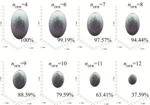
图 4 Screening ratios and envelope ellipsoid models from effective data realized by different DFR
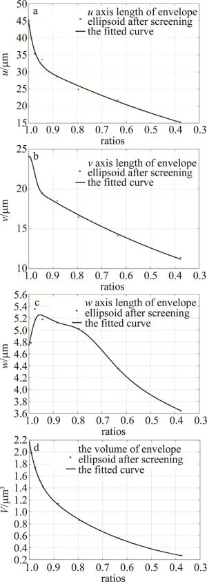
图 5 Characteristic changes of envelope ellipsoid with different screening ratios
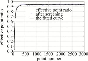
图 6 Change curve of the screening ratio with the total number of samples when DFR is 8
-
对于筛选后的有效数据,采用PSO进行最小包络椭球计算。在计算中,模型中粒子运动惯性因子ω=1,学习因子c1=c2=0.2,空间放大系数l0=15,逃逸系数es=2,粒子数为30个。
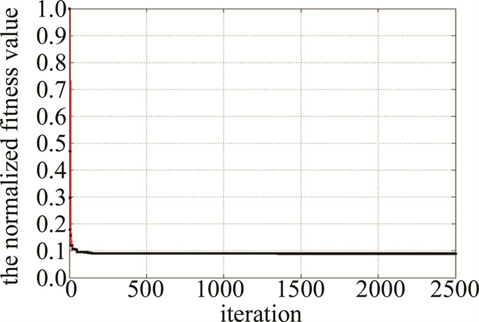
选取终止条件为计算到达最大迭代次数T=100000,包络比例re=0.99进行模型收敛测试。在Intel i5-6400 CPU 2.7GHz与8GB内存条件下,孤立森林筛选与最小包络椭球计算共耗时约为16.5min,其适应值的归一化收敛曲线如图 7所示。本次计算迭代到达5156次即实现最终收敛。以最终收敛结果为标准,本次计算迭代达到1354次时,收敛率达到99.88%,迭代达到2116次时,收敛率达到99.96%。据此,在最小包络椭球计算中,其终止条件可以设为达到最大迭代次数T=10000,经测试在上述计算设备条件下耗时不高于2min。在快速计算中,其终止条件可以设为最大迭代次数T=3000,经测试在上述计算设备条件下耗时不高于50s。
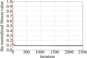
图 7 Convergence process of fitness value in minimum envelope ellipsoid calculation(within 2500 iterations)
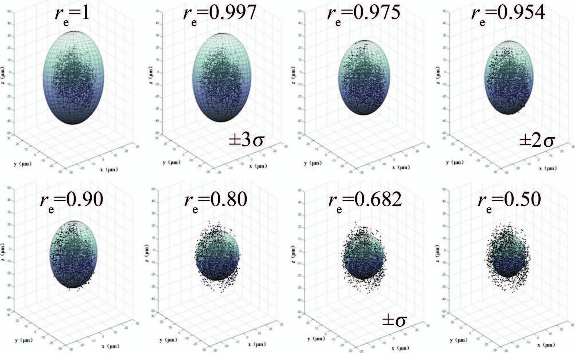
在实际测量测试中,会根据测量需求的精度要求选取由椭球中心向外不同置信区间进行测量规划设计,而最小椭球包络算法同样可以支持不同包络比例的不确定度范围计算,如此可以更直观地描述3维不确定度的概率密度分布。如图 8所示,当re=1时,即所有经筛选后的点全包络,减小re取值可以得到相应比例包络条件下的不确定度椭球模型。图 9为不同包络比例下椭球模型的体积变化,其拟合为双高斯分布。在包络比例re≈0.975时,其包络范围即为核心点云区域,这与系列模型研究相符[7]。
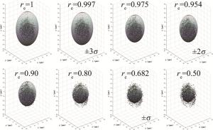
图 8 Minimum envelope ellipsoid model with different envelope ratios
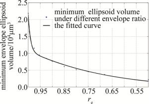
图 9 Curve of minimum envelope ellipsoid volume with different envelope ratios
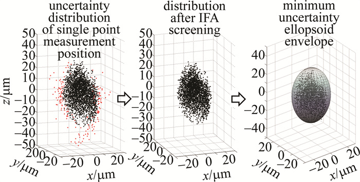
基于以上分析,图 10即为基于最小椭球包络的不确定度模型的计算方法流程: (1)针对特定点进行点云测量/仿真;(2)孤立森林算法采样点筛选;(3)进行PSO不确定度椭球包络模型建立。以此方法,距离4.7m的位置的共计3091个点测量数据,经过nDFR=8条件下的孤立森林算法筛选保留了2912个有效数据;通过re=0.975包络比例的粒子群10000次计算迭代,最终最小不确定度椭球包络三轴长为:a=4.95μm,b=18.39μm,c=30.53μm;计算总耗时121s。
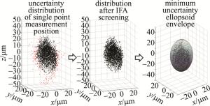
图 10 Calculation method of uncertainty model based on minimum ellipsoid envelope
-
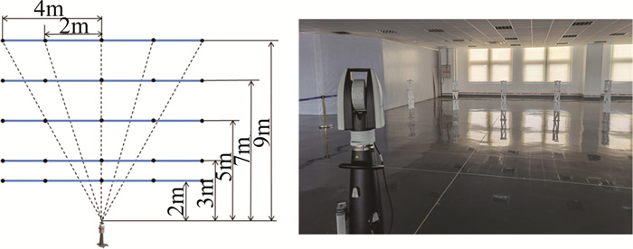
为直观测量空间中各位置激光跟踪仪的不确定度分布,设计了如图 11所示的实验。固定跟踪仪机位,在测量场地内规划处不同距离与测量方位的测量点;每个测量点以相同高度(约1.2m)固定靶座;对每个测量点分别进行多次重复测量;对每个测量位置的点云进行孤立森林筛选;筛选后的点云转移到该点位的UCS下进行PSO最小包络椭球模型计算;将获取的最小包络椭球转换到统一的MCS下,即得到空间各位置的不确定度分布。如图 12所示,为了方便直观观察各位置的不确定度椭球形貌与姿态,图中的不确定度椭球以6000倍轴长呈现。图 12a为测量空间的俯视图,可以看到,不确定度椭球的空间姿态得到了很好的还原;从图 12b可直观看到,该空间内不同位置的椭球尺寸变化,不确定度最主要受测量距离的影响。
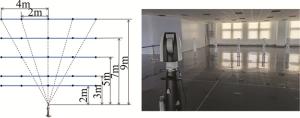
图 11 Experiment design of uncertainty test of laser tracker
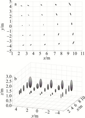
图 12 Uncertainty ellipsoid model distribution of different measurement positions (displayed by ellipsoid axis length magnified 6000×)
-
针对激光跟踪仪测量系统建立了其不确定度椭球模型,构建了面向椭球包络计算的不确定度椭球坐标系与面向场景分析的测量场坐标系,并提出了通用的转化模型。基于孤立森林算法构建了面向大量测量/仿真数据的有效数据筛选模型。基于粒子群优化算法建立了面向筛选后数据的最小椭球包络计算模型。针对当前航天有效载荷与天线系统大量应用的10m尺度量集,开展了特定点数据测量与测量场地不同位置的测量数据的分析与计算。模型高效准确地将测量的点云数据转化成特定点的不确定度椭球模型,并再现了其在测量场内的分布与姿态,这充分验证了数据筛选与最小椭球包络模型的有效性,也证明了模型的在不同条件下的适用性。这对高效快速准确地获取激光测量设备在3维测量空间内的测量不确定度分布情况,并对进一步完成高效地测量布局分析、设计研究具有重要意义。
该模型在针对其它激光球坐标测量系统、更大尺度量级以及面向多站、转站以及多系统联测角度的不确定度分析中均具有很强的应用潜力,这也是后续研究开展的重要方向。
激光测量系统不确定度最小包络椭球模型研究
Research on uncertainty minimum ellipsoid envelope model of laser measurement system
-
摘要: 为了对激光测量系统的测量误差3维空间分布进行有效评估, 以特定点测量或仿真的大量位置数据为基础, 采用孤立森林算法对点云进行了异常数据筛除。基于误差椭球理论, 引入粒子群优化算法, 针对有效数据建立了最小包络椭球的不确定度模型; 采用测量场与单点不确定度的坐标系变换, 将不确定度最小包络椭球模型应用于测量场景内不确定度场的空间分布分析; 通过单点以及10m量级范围空间场景实测数据的测试, 该模型可以高效地筛选有效采样数据, 并依据需求进行不同程度的最小包络椭球计算, 得到相应的不确定度。结果表明, 基于测量位置数据, 该模型可以高效准确地描述单点位置的3维不确定度范围, 并能够有效地再现测量空间内的不确定度分布, 在4.7m的测量距离、94.2%的筛选后有效数据、97.5%的包络比例下, 计算获得不确定度范围为三轴长4.95μm, 18.39μm和30.53μm的椭球。该最小包络椭球不确定度模型在基于实测的理论模型验证、设备状态与测量场景环境分析, 以及测量布局设计等方面具有着重要的价值。Abstract: In order to effectively evaluate the three-dimensional spatial distribution of measurement errors of the laser measurement system, a new uncertainty model based on the calculation of the minimum envelope ellipsoid was proposed. Based on the measured or simulated location data, the isolated forest algorithm was introduced to filter out abnormal data in the point cloud. With the valid data, the minimum envelope ellipsoid uncertainty model was established based on the particle swarm optimization and the error ellipsoid theory. By the coordinate system transformation between the measurement field and the single point uncertainty, the minimum envelope ellipsoid model was applied to the spatial uncertainty distribution analysis. Through the test of the measured data of a single point and a 10m-level space scene, the model can efficiently screen the sampling data and perform different levels of minimum envelope ellipsoid calculations according to the requirements. And then the corresponding uncertainty can be obtained. The results show that based on the measurement position data, the model can efficiently and accurately describe the three-dimensional uncertainty range of a single point position, and can effectively reproduce the uncertainty distribution in the measurement space. With the experimental conditions of a measurement distance 4.7m, the effective data after screening 94.2%, and an envelope ratio 97.5%, an ellipsoid with an uncertainty range of three-axis length 4.95μm, 18.39μm, 30.53μm is obtained by the model calculation. The minimum envelope ellipsoid uncertainty model has important value in many aspects, such as theoretical model verification based on actual measurement, equipment state and measurement environment analysis, and measurement layout design.
-
图 4 Screening ratios and envelope ellipsoid models from effective data realized by different DFR
图 6 Change curve of the screening ratio with the total number of samples when DFR is 8
图 7 Convergence process of fitness value in minimum envelope ellipsoid calculation(within 2500 iterations)
-
[1] SWYT D A. Length and dimensional measurements at NIST[J]. Journal of research of the National Institute of Standards and Techno-logy, 2001, 106(1): 1-23. doi: 10.6028/jres.106.002 [2] SHI H Y, GUO T, WANG D, et al. Power line suspension point location method based on laser point cloud[J]. Laser Technology, 2020, 44(3): 364-370(in Chinese). [3] SUI Sh Ch, ZHU X Sh. Digital measurement technique for evaluating aircraft final assembly quality[J]. Scientia Sinica Technologica, 2020, 50: 1449-1460(in Chinese). doi: 10.1360/SST-2020-0049 [4] DENG Zh P, LI S G, HUANG X. Coordinate transformation uncertainty analysis and reduction using hybrid reference system for aircraft assembly[J]. Assembly Automation, 2018, 38(4): 487-496. doi: 10.1108/AA-08-2017-097 [5] MEI Z, MAROPOULOS P G. Review of the application of flexible, measurement-assisted assembly technology in aircraft manufacturing[J]. Proceedings of the Institution of Mechanical Engineers, 2014, B228(10): 1185-1197. [6] CHEN Z H, DU F Zh, TANG X Q. Research on uncertainty in mea-surement assisted alignment in aircraft assembly[J]. Chinese Journal of Aeronautics, 2013, 26(6): 1568-1576. doi: 10.1016/j.cja.2013.07.037 [7] DENG Zh Ch, WU Zh Y, YANG J G. Point cloud uncertainty analysis for laser radar measurement system based on error ellipsoid model[J]. Optics and Lasers in Engineering, 2016, 79: 78-84. doi: 10.1016/j.optlaseng.2015.11.010 [8] COX M G, HARRIS P M. Measurement uncertainty and traceability[J]. Measurement Science and Technology, 2006, 17(3): 533-540. doi: 10.1088/0957-0233/17/3/S13 [9] ZHANG F M, QU X H. Fusion estimation of point sets from multiple stations of spherical coordinate instruments utilizing uncertainty estimation based on Monte Carlo[J]. Measurement Science Review, 2012, 12(2): 40-45. [10] REN Y, LIN J R, ZHU J G, et al. Coordinate transformation uncertainty analysis in large-scale metrology[J]. IEEE Transactions on Instrumentation and Measurement, 2015, 64(9): 2380-2388. doi: 10.1109/TIM.2015.2403151 [11] ZHU J K, LI L J, LIN X Zh. Research on the measurement field planning of lidar measurement system[J]. Laser Technology, 2021, 45(1): 99-104(in Chinese). [12] BERGSTRÖM P, EDLUND O. Robust registration of point sets using iteratively reweighted least squares[J]. Computational Optimization and Applications, 2014, 58(3): 543-561. doi: 10.1007/s10589-014-9643-2 [13] WANG Q, HUANG P, LI J X, et al. Uncertainty evaluation and optimization of INS installation measurement using Monte Carlo method[J]. Assembly Automation, 2015, 35(3): 221-233. doi: 10.1108/AA-08-2014-070 [14] JIN Zh J, YU C J, LI J X, et al. Configuration analysis of the ERS points in large-volume metrology system[J]. Sensors, 2015, 15(9): 24397-24408. doi: 10.3390/s150924397 [15] PREDMORE C R. Bundle adjustment of multi-position measurements using the Mahalanobis distance[J]. Precision Engineering, 2010, 34(1): 113-123. doi: 10.1016/j.precisioneng.2009.05.003 [16] CALKINS J M. Quantifying coordinate uncertainty fields in coupled spatial measurement systems[D]. Virginia, USA: Virginia Polytechnic Institute and State University, 2002, 1: 48. [17] LIU Y, SUN Sh Y. Laser point cloud denoising based on principal component analysis and surface fitting[J]. Laser Technology, 2020, 44(4): 497-502(in Chinese). [18] CHEN H S, MA H Zh, CHU X N, et al. Anomaly detection and critical attributes identification for products with multiple operating conditions based on isolation forest[J]. Advanced Engineering Informatics, 2020, 46: 101139. doi: 10.1016/j.aei.2020.101139 [19] SUSTO G A, BEGHI A, MCLOONE S. Anomaly detection through on-line isolation Forest: An application to plasma etching[C] // Proceeding of the 28th Annual SEMI Advanced Semiconductor Ma-nufacturing Conference (ASMC). New York, USA: IEEE, 2017: 89-94. [20] LIU F T, TING K M, ZHOU Zh H. Isolation-based anomaly detection[J]. ACM Transactions on Knowledge Discovery from Data, 2012, 6(1): 1-39. [21] CHEN W R, YUN Y H, WEN M, et al. Representative subset selection and outlier detection via isolation forest[J]. Analytical Methods, 2016, 8(39): 7225-7231. doi: 10.1039/C6AY01574C [22] KENNEDY J, EBERHART R. Particle swarm optimization[C] // Proceeding of IEEE International Conference on Neural Networks. New York, USA: IEEE, 1995: 1942-1948. [23] POLI R, KENNEDY J, BLACKWELL T. Particle swarm optimization[J]. Swarm Intelligence, 2007, 1(1): 33-57. doi: 10.1007/s11721-007-0002-0 [24] ALAM S, DOBBIE G, KOH Y S, et al. Research on particle swarm optimization based clustering: A systematic review of literature and techniques[J]. Swarm and Evolutionary Computation, 2014, 17: 1-13. doi: 10.1016/j.swevo.2014.02.001 [25] LI Y, XING Y, FANG C, et al. An experiment-based method for focused ion beam milling profile calculation and process design[J]. Sensors and Actuators, 2019, A286: 78-90. [26] LI Y, GOSÁLVEZ M A, PAL P, et al. Particle swarm optimization-based continuous cellular automaton for the simulation of deep reactive ion etching[J]. Journal of Micromechanics and Microengineering, 2015, 25(5): 055023. doi: 10.1088/0960-1317/25/5/055023 [27] CHEN S Q, ZHANG H Y, ZHAO Ch M, et al. Point cloud registration method based on particle swarm optimization algorithm improved by beetle antennae algorithm[J]. Laser Technology, 2020, 44(6): 678-683(in Chinese). -

 点击查看大图
图(13)
计量
- 文章访问数: 7415
- HTML全文浏览量: 4089
- PDF下载量: 33
- 被引次数: 0
